Here’s a search query: “beach trip.”
Full-text search finds nothing — no record contains the word “beach.” But there’s a note that says “Qué calor en Valencia, el agua estaba perfecta.” Semantic search finds it because the embedding for “beach trip” is close to the embedding for a hot day at the beach in Valencia.
Now a different query: “Ana García.”
Semantic search returns a dozen vaguely related records. Full-text search returns the 3 records that literally contain “Ana García.” But neither shows you that Ana attended last week’s meeting, is CC’d on 5 email threads, and appears in tomorrow’s calendar — connections that only the knowledge graph knows about.
No single search method is enough. We needed all three, plus a way to combine them that doesn’t require manual tuning.
The four signals
Our search pipeline produces four independent scores for every candidate result:
| Signal | Source | What it catches | Tier |
|---|---|---|---|
| Semantic | pgvector cosine similarity | Meaning-based matches (“beach” → “calor en Valencia”) | Pro |
| Full-text | tsvector + GIN + ts_rank | Exact keyword matches, fast and precise | Free |
| Graph | entity_links overlap | Relational connections (“Ana García” → meetings she attended) | Pro |
| Heat | record_heat table | Temporal relevance (recently accessed records) | Free (display), Pro (in ranking) |
Free tier users get full-text search only — which is still fast and well-ranked thanks to tsvector with weighted columns (title gets weight A, content gets weight B, tags get weight C). Pro users get all four signals fused together.
The pipeline
The search happens in seven steps:
Query: "Ana García project update"
    │
    ├── 1. Vector search ──→ top-50 by cosine similarity
    ├── 2. Full-text search ──→ top-N by ts_rank (UNION ALL across domains)
    └── 3. Graph discovery ──→ N candidates via entity_links
                │
                ▼
         4. Deduplicate by (domain, record_id)
                │
                ▼
         5. Rank-normalize each signal to [0, 1]
                │
                ▼
         6. Detect degenerate signals
                │
                ▼
         7. Weighted fusion + multi-signal bonus
                │
                ▼
            Final ranked results with provenance
Let me walk through each step.
Step 1: Vector search
The query text is embedded on-the-fly using the same model that embeds records (qwen3-embedding:0.6b, 1024 dimensions). Then a cosine similarity query runs against the embeddings table:
SELECT domain, record_id, 1 - (embedding <=> $query_embedding) AS similarity
FROM embeddings
WHERE 1 - (embedding <=> $query_embedding) >= 0.3
ORDER BY embedding <=> $query_embedding
LIMIT 50;
The 0.3 minimum threshold filters garbage. The top 50 candidates move to the next step. If Ollama is down and we can’t embed the query, this signal is simply skipped — the other signals still work.
Step 2: Full-text search
A UNION ALL query across all domain tables, using PostgreSQL’s native full-text search:
SELECT 'note' AS domain, id AS record_id, ts_rank(search_vector, query) AS score
FROM notes
WHERE search_vector @@ plainto_tsquery('simple', $q) AND deleted_at IS NULL
UNION ALL
SELECT 'event', id, ts_rank(search_vector, query)
FROM events
WHERE search_vector @@ plainto_tsquery('simple', $q) AND deleted_at IS NULL
UNION ALL
-- ... contacts, emails, files, diary, bookmarks, kanban_cards
ORDER BY score DESC
LIMIT 50;
We use plainto_tsquery('simple', ...) instead of language-specific configurations. The simple configuration doesn’t stem words, which matters for multilingual data — Spanish and English records coexist, and stemming rules for one language would butcher the other.
Each domain table has a search_vector tsvector column maintained by a trigger (or GENERATED ALWAYS AS ... STORED for newer tables). The vectors are weighted: title gets 'A', description/content gets 'B', tags get 'C'. A match in the title ranks higher than a match in the body.
Step 3: Graph discovery
This signal is different — it doesn’t match text, it matches relationships.
The query is matched against graph_entities.normalized_name. If “Ana García” matches a Person entity, we find all records linked to that entity via entity_links:
-- Find entities mentioned in the query
SELECT id FROM graph_entities
WHERE normalized_name ILIKE '%ana garcia%' AND deleted_at IS NULL;

-- Find all records linked to those entities
SELECT source_type AS domain, source_id AS record_id
FROM entity_links
WHERE target_type = 'graph_entity' AND target_id = ANY($entity_ids);
The graph_score for each result is the overlap ratio: how many of the query’s entities appear in the result’s connections, divided by the total entities found in the query.
Step 4: Deduplication
The three signals produce candidate sets that overlap. A note containing “Ana García” might appear in vector search (semantically similar), full-text search (exact keyword match), and graph search (linked to the Ana García entity). We deduplicate by (domain, record_id) and track which signals produced each candidate.
Step 5: Rank-based normalization
Here’s where it gets interesting. We do NOT normalize by raw scores. We normalize by rank position:
normalized_value = (N - position) / NThe top result in a signal gets 1.0. The bottom gets nearly 0. A candidate absent from a signal gets 0.
Why rank-based instead of min-max normalization? Because cosine similarity scores cluster. In a typical query, the top-50 vector search results might have similarities between 0.54 and 0.64 — a 10-point range. Min-max normalization would stretch this to 0.0–1.0, making the difference between rank 1 and rank 50 look huge when it’s actually tiny.
Rank-based normalization treats position as the signal, not magnitude. First place is first place, whether it scored 0.99 or 0.55.
Step 6: Degenerate signal detection
Sometimes a signal doesn’t discriminate. If all 50 vector search results have cosine similarities within 5% of each other, the signal is noise — everything “looks the same” to the embedding model.
When this happens, the weight assigned to the degenerate signal gets redistributed proportionally to the other signals. The search doesn’t fail — it just relies more on the signals that are actually informative.
Step 7: Weighted fusion + multi-signal bonus
The final score combines all four signals:
score = (α × heat + β × semantic + γ × fulltext + δ × graph) / (α + β + γ + δ)Default weights: all equal at 0.25 each. But the user can adjust them via the dashboard’s ranking sliders — crank heat to prioritize recent activity, drop graph to ignore relationship signals, etc.
Then comes the multi-signal bonus:
| Signals that found this result | Multiplier |
|---|---|
| 1 signal only | ×1.00 |
| 2 signals | ×1.25 |
| 3 signals | ×1.50 |
A result that appears in vector search, full-text search, AND graph search gets a 50% bonus. This rewards results that are independently confirmed by multiple methods — they’re almost certainly relevant.
Heat doesn’t count for the bonus calculation. It’s a temporal signal, not a relevance signal — a record being hot doesn’t mean it matches the query.
Two search modes
The system exposes two search endpoints that use this pipeline differently:
Standard search: GET /search
The default. Uses Reciprocal Rank Fusion with fixed weights:
rrf_score = Σ 1/(K + rank_i)    where K = 60
final = rrf_score × (1 + 0.1 × heat_score)
RRF is elegant: it ignores raw scores entirely, only caring about rank position. A result that’s #1 in vector search and #3 in full-text search gets 1/(60+1) + 1/(60+3) = 0.0164 + 0.0159 = 0.0323. The K=60 constant smooths the curve — the difference between rank 1 and rank 10 is meaningful but not extreme.
Heat acts as a post-fusion tiebreaker with a maximum 10% boost. It never dominates relevance. A cold but highly relevant result always beats a hot but marginally relevant one.
Advanced search: GET /search/advanced
The full power mode. Four independent sliders, degenerate signal detection, multi-signal bonus. Used by the Search module in the dashboard where users can see and control exactly how results are ranked.
Every result includes full provenance:
{
  "provenance": {
    "heat_score": 0.52,
    "vector_score": 0.68,
    "fulltext_score": 0.52,
    "graph_score": 0.11
  }
}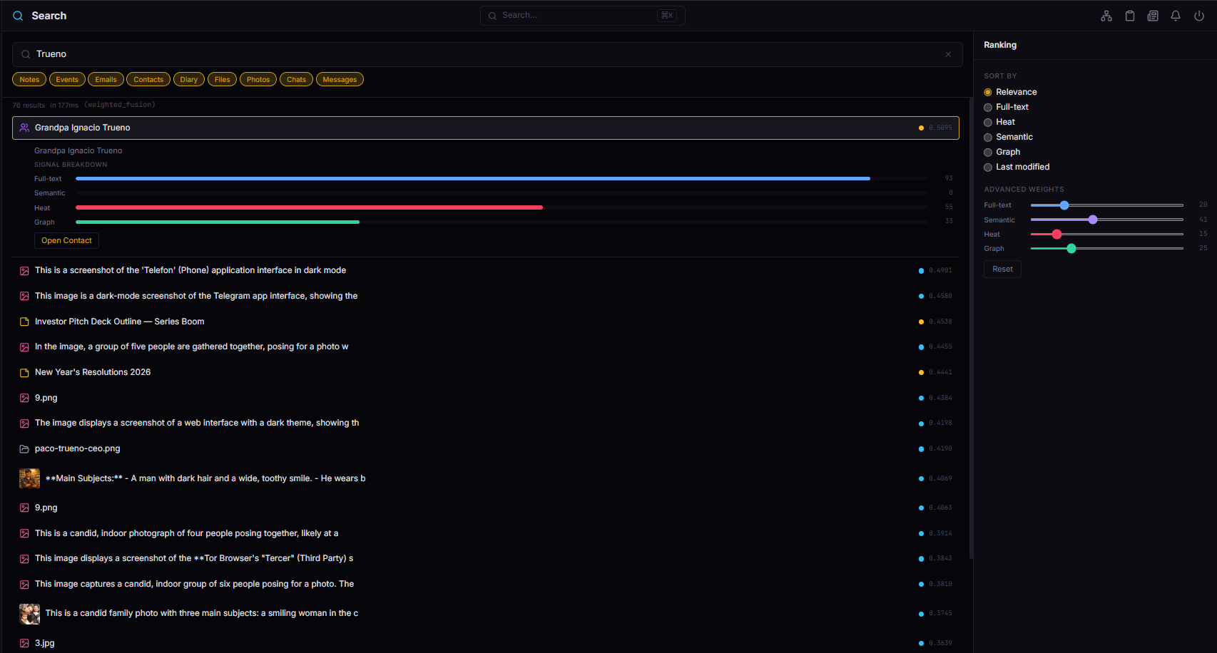
Complete transparency. The user can see that a result ranked high because of semantic similarity (0.68) despite low graph connectivity (0.11), and adjust weights accordingly.
Free tier: surprisingly good without vectors
Free users don’t get semantic search, graph search, or heat-weighted ranking. They get tsvector + GIN full-text search across all domains, with ts_rank() scoring and weighted columns.
This sounds like a big downgrade. In practice, it’s surprisingly solid:
- Searches for names, titles, and specific terms work perfectly — full-text search is exact.
- Weighted tsvector means a match in the title ranks above a match in the body.
plainto_tsquery('simple', ...)handles both Spanish and English without configuration.- The UNION ALL across domains means one search bar finds notes, emails, events, contacts, and files.
- GIN indexes make it O(log n) — fast even with tens of thousands of records.
The meaningful Pro differentiator is semantic search: finding “calor en Valencia” when you search for “beach trip.” That’s genuinely impossible with keyword matching. But for the 80% of searches where people type exactly what they’re looking for, free tier search works fine.
Temporal expansion: the “wow” moment
Here’s a feature that surprised us with how useful it turned out to be.
If the query mentions an entity that has upcoming events (within ±7 days), temporally close results get a boost:
temporal_boost = 1 + 0.15 × proximityIn practice: you search for “Ana García.” The system finds that Ana has a meeting with you tomorrow. Notes, emails, and contacts related to Ana that were created or accessed in the last week get boosted. The search results naturally organize around “here’s everything relevant to Ana before your meeting tomorrow.”
We didn’t plan this as a feature — it fell out of having the knowledge graph and the calendar in the same database. But it consistently produces the kind of results that make people say “how did it know I needed that?”
The tuning knobs
Five parameters control the pipeline behavior:
| Parameter | Default | What it does |
|---|---|---|
MIN_SIMILARITY | 0.3 | Cosine sim threshold. Higher = less vector noise |
RRF_FETCH_SIZE | 50 | Candidates per signal. Lower = faster, fewer candidates |
RRF_K | 60 | RRF smoothing constant. Higher = smoother rank differences |
| Multi-signal factor | 0.25 | Bonus per additional signal (1 + 0.25 × (count-1)) |
| Degenerate threshold | 5% | Signal suppression when score range is too narrow |
We’ve left these at their defaults since implementation. The multi-signal bonus and degenerate detection handle most edge cases automatically. If we ever need to tune, the provenance metadata on every result tells us exactly which signal is helping or hurting.
Performance
All of this runs inside a single PostgreSQL instance, on the same machine that serves the API:
| Operation | Latency |
|---|---|
| Vector search (50 candidates) | ~15-30ms |
| Full-text search (UNION ALL, 7 tables) | ~5-15ms |
| Graph discovery | ~5-10ms |
| Fusion + scoring | ~2-5ms |
| Total (standard search) | ~30-60ms |
| Total (advanced search, 4 signals) | ~50-80ms |
No Elasticsearch. No Solr. No separate search service. pgvector and tsvector are PostgreSQL extensions that run in the same process as the rest of the database. One backup strategy, one connection pool, one operational concern.
For a personal system with a few thousand records per domain, this is more than fast enough. If we ever hit scale problems (unlikely for single-user), the first optimization would be reducing RRF_FETCH_SIZE from 50 to 20 — cutting candidate generation in half with minimal quality loss.
What I’d do differently
I’d implement full-text search from the very beginning, not as a free-tier afterthought. We built vector search first (Phase 3) and added tsvector later as a “fallback for free users.” Turns out full-text search is essential even for Pro users — it catches exact matches that embeddings miss. “Show me the email from [email protected]” is a full-text query, not a semantic one.
I’d add provenance to the standard search too, not just advanced. We initially only exposed the score breakdown in /search/advanced. When we added it to the standard /search endpoint (in the provenance field), debugging search quality became ten times easier. Every bug report went from “the search is bad” to “this result has vector_score 0.8 but graph_score 0, why?”
I’d explore reranking with a cross-encoder. Our pipeline does retrieval + fusion but no reranking. A small cross-encoder model (like ms-marco-MiniLM) could re-score the top 20 results for higher precision. We deferred this because the current quality is good enough and adding another model to the Ollama queue would increase latency. But for a future post-MVP iteration, it’s the obvious next step.
The takeaway
The trick to hybrid search isn’t the individual signals — pgvector and tsvector are well-documented, and knowledge graph traversal is just recursive CTEs. The trick is the fusion: how you combine signals with different scales, different failure modes, and different strengths.
Reciprocal Rank Fusion solves the scale problem — ranks instead of raw scores. Degenerate signal detection solves the failure mode problem — a noisy signal gets suppressed instead of poisoning results. Multi-signal bonus solves the confidence problem — results confirmed by multiple methods are almost certainly good.
Four signals, one UNION ALL, one PostgreSQL instance, under 100ms. The search that finds “calor en Valencia” when you type “beach trip” — and also shows you that Ana García has a meeting with you tomorrow.
Next up: sleep-time compute for personal data — what your AI should be doing while you sleep, and why idle cycles are the most valuable compute you have.